The Land Survey Misclose ~ a perfection of plane trigonometry and coordinate geometry, as applied to cadastral survey practice.
For Gillian ~
Who really wanted to know
And was there from the beginning.
.
The land survey close computation is fundamental to the development of the cadastre. A primary element of the Torrens Title land system is the inclusion of a title diagram reference in the issued Certificate of Land Title. In New South Wales, a plan of survey of the land parcel prepared by a Registered Land Surveyor, meets the requirements of a title diagram.
The external perimeter boundaries of a land parcel are delineated in a plan of survey by lines, each line being annotated with a bearing and a distance. The accuracy and correctness of these stated measurements can be mathematically confirmed by the undertaking of a survey close computation.
.

.A diagram example of a plan of survey showing a green triangle shaped land parcel, comprising three ground points, with bearing and distance measurements detailed on the three red perimeter boundary lines. These red lines may also be referred to as a closed traverse loop.
Background
In the mid-1960s, closed traverse computations were undertaken with the use of printed trigonometrical tables and a mechanical calculator. The introduction of scientific programmable RPN calculators in the early 1970s, took the tedium out of the survey close computation process. Current personal computer technology again dramatically improved survey computations through the use of purpose COGO and CAD software programs.
Increased computing power for land survey computations, lead to a move away from grid subdivision layouts to curvilinear land developments, blending in more with the topography.
Precision field measurement of lines between ground points, are accurately measured with modern total station instrumentation. Angles or bearings and distances are measured electronically. Distances measured are slope distances, subsequently reduced to the horizontal, and observed bearings are directions of lines relative to a map grid north.
For further reference reading, see my previously published article titled ~ Surveying computations and the land boundary Surveyor.
How the survey close computation works
A point position on a plane surface may be defined by rectangular coordinates, being an East and North coordinate value. For Pt. 1 in the diagram, coordinates East 500.000 metres and North 500.000 metres, are arbitrarily set as the start point values for this three line traverse.
The bearing and distance of each traverse line, through trigonometry, can be transformed into an orthogonal North – South axis and East – West axis distance component. View the three blue triangles edged in black in the diagram.
Computing N/S and E/W components for line 2 to 3
SIN 137° 10′ 20″ x 115.865 = 0.679797 x 115.865 = 78.764 ~ Easting component
COS 137° 10′ 20″ x 115.865 = – 0.733400 x 115.865 = – 84.975 ~ Southing component
.
Using these calculated N/S and E/W distance components, coordinates can be computed for all points sequentially, clockwise around the traverse loop.
Coordinates calculation for Pt. 2 ~ E 500.000 + 128.856 = E 628.856 ~ N 500.000 + 154.909 = N 654.909
Coordinates calculation for Pt. 3 ~ E 628.856 + 78.764 = E 707.620 ~ N 654.909 – 84.975 = N 569.934
Coordinates calculation back to start Pt. 1 ~ E 707.620 – 207.620 = E 500.000 ~ N 569.934 – 69.934 = N 500.000
.
The correctness and accuracy of the measured traverse loop can be checked by the comparison of the original starting coordinates, with coordinates generated sequentially through the traverse back to the initial starting point. The traverse misclose is the difference between the initial coordinates and final coordinates back to the starting point, generated through the traverse. For this traverse, the misclose is E 0.000 and N 0.000.
A typical “real life” survey misclose for the traverse loop, as shown in the diagram, would be of the order of about 0.025 metres. This is conventionally expressed as the ratio of about 1 : 21,450, which meets the criteria for a rural land boundary survey. The ratio represents the misclose related to the traverse loop perimeter.
.

A screenshot of a DOS based survey close computation, PC software vintage about 1990, showing the traverse computation close of the red sided triangle.
.

Screenshot from CDS Version 2.3 software, 2011, showing listing output for the red triangle traverse diagram.
.

Screenshot of the HP 15c Scientific RPN Programmable Calculator, first available in about 1983.
HP 15c RPN programmable calculator, old technology at its best. Find as a PDF attachment, my instructions in the use of a HP 15c in undertaking a survey close traverse computation, together with the necessary program steps to be inputted in the HP 15c, to enable the running of this Survey Close program.
Something for future consideration ~ the mathematics of a triangle on a curved surface, as applied to the astronomical triangle. Watch this blog.
Acknowledgements:
Under my gentle supervision and direction, Gillian road tested all the necessary survey computations in the preparation of this article, as well as undertaking all the transcriptions. Well done GFP. Gillian absorbed and learnt a lot, but no exams required !
Special thanks to Sam, our computer guru, who introduced us to VIRTUAL BOX, which enabled the use of Windows XP in a macOS Monterey environment. This permitted the running of my old land survey software on an iMac PC.
References:
Foxall, H.G., Handbook for Practising Land and Engineering Surveyors, Pub. 1957, NSW Institution of Surveyors, Sydney.
CDS Professional Solutions, Civil Design & Survey software, CDS 2.3, March 2011.
Mackie, J.B., The Elements of Astronomy for Surveyors, Pub. 7th edition 1971, Charles Griffin & Co., London.
HP 15c Scientific RPN Calculator app, Apple macOS Monterey, App Store.
Triangle Solver app, designed for iPad and iPhone, iOS 9.0 or later, App Store.
.

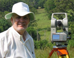
Time before ~
An elated and exhausted Gillian walking out of a rural survey job in the Byron Hinterland. Note the extendable prism pole, holding an attached mini reflecting prism, with the Sokkia Total Station instrument in the left corner foreground. Again, Gillian at her surveying best. Photo taken by Robert.